Probability distributions

Random variable

• A variable that can produce possible values those are outcomes of a random experiment is called random variable.
• Types:
  • Discrete random variable is a random variable that has countable number of possible values.
    • Example: Random variable representing the sum of 2 dices.
  • Continuous random variable is a random variable where the data can be infinitely random.
    • Example: Random variable representing the height of students in a class.

Probability distribution

• It is a table of values that shows the probabilities of all possible values of a random variable.
• Probability distribution for discrete and continuous are different.

Example 1

• Let’s take an example of rolling 2 dices simultaneously.
• Let X be a random variable representing the sum of 2 dices.
• All the possible values of X are 2, 3, 4, 5, 6, 7, 8, 9, 10, 11, 12

• Let’s tabulate the probabilities for all possible values of X:

  X	2	3	4	5	6	7	8	9	10	11	12
  P(X)	$\dfrac{1}{36}$	$\dfrac{2}{36}$	$\dfrac{3}{36}$	$\dfrac{4}{36}$	$\dfrac{5}{36}$	$\dfrac{6}{36}$	$\dfrac{5}{36}$	$\dfrac{4}{36}$	$\dfrac{3}{36}$	$\dfrac{2}{36}$	$\dfrac{1}{36}$

• Probability distribution

  

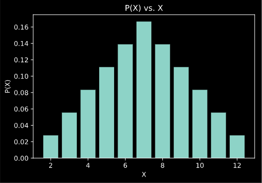
  The chart above is the probability distribution of a discrete random variable. In this case, the discrete random variable (X) is the sum of two dice.

Example 2

• Given, the discrete probability distribution of a biased dice is:

  Number	1	2	3	4	5	6
  Probability	$\dfrac{1}{12}$	$\dfrac{1}{6}$	$\dfrac{1}{4}$	$\dfrac{1}{4}$	$\dfrac{1}{6}$	$\dfrac{1}{12}$

• $$\begin{align*} \text{Mean }(\mu) = & \sum x \cdot P(x) \\ = & 1 \cdot \dfrac{1}{12} + 2 \cdot \dfrac{1}{6} + 3 \cdot \dfrac{1}{4} \\ & + 4 \cdot \dfrac{1}{4} + 5 \cdot \dfrac{1}{6} + 6 \cdot \dfrac{1}{12} \\ = & 3.5 \end{align*}$$
• $$\begin{align*} Variance = & \sum [ \, (x - \mu)^2 \cdot P(x) ] \, \\ = & (1 - 3.5)^2 \cdot \dfrac{1}{12} \\ & + (2 - 3.5)^2 \cdot \dfrac{1}{6} \\ & + (3 - 3.5)^2 \cdot \dfrac{1}{4} \\ & + (4 - 3.5)^2 \cdot \dfrac{1}{4} \\ & + (5 - 3.5)^2 \cdot \dfrac{1}{6} \\ & + (6 - 3.5)^2 \cdot \dfrac{1}{12} \\ = & 1.886 \end{align*}$$
• $$\begin{align*} \text{standard deviation }(\sigma) & = \sqrt{variance} \\ & = \sqrt{1.886} \\ & = 1.373 \end{align*}$$

Probability mass function (PMF)

• A function, say, P is said to be a probability mass function for a random discrete variable X when P(X) gives the value of the probability of X.
• In the example above, P(2) is equal to 1/36, where P is the PMF of the discrete random variable X, which is the sum of two dice.

Discrete Probability Distribution

1. Binomial distribution

• It is applied to discrete data when there are only 2 possible outcomes of any event that are labelled as Success or Failure.
• It is used to calculate the probability of getting a fixed number of successes in a given number of trials.
• PMF of Binomial distribution:
  $P(x) = \dfrac{n!}{x! \cdot (n-x)!} \cdot p^x \cdot q^{n-x}$
  where,
  • n = the number of trials
  • x = the number of successes desired
  • p = the probability of getting a success in one trial
  • q = the probability of getting a failure in one trial

2. Bernoulli distribution

• Special case of Binomial distribution where the number of trials(n) is equal to 1. Like binomial distribution, there are 2 possible outcomes (labelled as success and failure) of a trial. The value of the random variable X is taken as 1 when a success occurs, and it is taken as 0 when a failure occurs.
• PMF of Bernoulli distribution:
  $P(x) = p^x \cdot (1-p)^{1-x}$
  where,
  • p = probability of success
  • x = 1(for success) and 0(for failure)
• Bernoulli distribution is used to model a single individual that is experiencing events having 2 outcomes like death and disease.

3. Poisson distribution

• It is used to calculate the probability of a given number of events occurring in the fixed intervals of time.
• PMF for Poisson distribution:
  $P(x) = \dfrac{\lambda^x \cdot e^{-\lambda}}{x!}$
  where,
  • x = the number of occurrences per time interval
  • $\lambda$ = average
• Example: Suppose that, in a shop, customers arrive randomly on weekdays at an average of 5 customers every hour. What is the probability that exactly 8 customers will arrive in an hour on a weekday? Here,
  $\lambda = 5$
  $x = 8$
  $P(x = 8) = \dfrac{5^8 \cdot e^{-5}}{8!}$
  As we can see that Poisson distribution is used to forecast the number of customers or sales on certain days or seasons of the year. This forecast can help businessman maintain stock according to the demand.
• Example:
  Suppose that from a warehouse of lathe machines, an average of 5 units of machines leave the warehouse per week. At the end of every week, 5 units of machines are bought from the assembler and stored in the warehouse. Having more machines in the warehouse increases the cost of maintenance and storage, and at any given time, the warehouse can store no more than 8 units. Calculate the probability of the following scenario:
  In a given week, less than 2 machines leave the warehouse. (In this situation, after the new batch of machines arrives from the assembler, the number of machines will exceed the warehouse capacity.)
  This can be solved by Poisson distribution:
  $P(x) = \dfrac{\lambda^x \cdot e^{-\lambda}}{x!}$, $\lambda = 5$
  P(x=0) + P(x=1) will give us the desired probability.
  $P(x=0) = \dfrac{5^0 \cdot e^{-5}}{0!} = 0.006$
  $P(x=1) = \dfrac{5^1 \cdot e^{-5}}{1!} = 0.033$
  $P(x<2) = 0.006 + 0.033 = 0.039$

Continuous Probability Distribution

• The probability distribution of a continuous random variable is called the Probability Density Function (P.D.F.).
• The curve below is a probability density function.
  
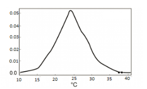
• Properties of P.D.F.:
  • The total area under the curve is 1
  • The probability that a Random variable X will lie between ‘a’ and ‘b’ is equal to the integration of the probability distribution function over a and b.
    $P(a \leq X \leq b) = \int_a^b f(x)dx$
    Here,
    • f(x) is probability density function
    • P(x) is cumulative distribution function
• The most common probability distribution is Normal distribution.