F-Test

Two sample t-tests can validate a hypothesis containing only two groups at a time. For samples involving three or more groups, the t-test becomes tedious as you have to perform the tests for each combination of the groups. Also, Type-1 error increases in this process. You use ANOVA in such cases.

ANOVA

ANOVA or Analysis of Variance can determine whether the means of three or more groups are different. ANOVA uses F-tests to statistically test the equality of means.

Let’s look an example to understand how ANOVA works:

A test was conducted in a workplace, and the feedback on the three e-commerce platforms was recorded in a dataset. Following is the dataset:

Amazon	Flipkart	Snapdeal
7.5	7	5
8.5	9.5	7.5
6	10	8.5
10	6	3
8.5	7.5	6
8	8.5	5
8	10	7
6	6.5
9.5	6.5
10	9
6.5	10

To begin with, create a null hypothesis for your ANOVA test. In this case:

• Your null hypothesis ($H_0$) will be — “All the platforms are equally popular”.
  • $H_0: \mu_1 = \mu_2 = ... = \mu_k$ (where k is the number of different populations or groups or treatment levels, in our case, it’s 3).
  • By writing above, you suggest that the mean of the different populations will be same, which is your null hypothesis.
  • If the above statement is proved at the end of your test, it will imply that all platforms are equally popular; otherwise you accept your alternate hypothesis ($H_1$).
• The alternate hypothesis ($H_1$), thus, becomes “At least one of the platforms has different popularity from the rest”.

The process is called analysis of ‘variance’ though you are comparing ‘means’ is because the math you will use later in the process will require the concept of variance to study the means of the groups. It will tell you how the means vary or differ.

Let’s briefly summarize variance:

Variance is the average squared deviation of a data point from the distribution mean. The distance between the sample mean and each data point is measured and squared. Then, you add it together and take the average. The formula is:

$$s^2 = \dfrac{\sum{(x - \overline{x})^2}}{n - 1}$$

Here,

• $s^2$ represents the variance
• x represents sample data points
• $\overline{x}$ represents the sample mean
• n is number of sample points

Sum of squares

You need two kinds of calculations that you have to make in accordance with the variance.

• Sum of squares between, SSB accounts for the variation between the groups, and
• sum of squares within, SSW accounts for the variation within a group.

• The total sum of squares, TSS is the sum of all the variations that there are, and it gives us the deviation of each observation from the grand mean of the dataset. To understand this more clearly, let’s look at your case:

• SSB represents the variation of the mean feedback of a company, say Flipkart, from the grand mean of all the feedback.
  • SST i.e. Treatment sum of squares is the variation attributed to, or in this case between, the companies.
  • It is same as SSB
• SSW represents the variation of all the feedback in a company from the mean of its feedback.
  • SSE i.e. Sum of squares of the residual error which is the variation attributed to the error.
  • It is same as SSW
• TSS represents the variation of all the feedback in your dataset from the grand mean.

Total sum of squares = Sum of squares between + Sum of squares within the group, or
$TSS = SSB + SSW$, or
Total sum of squares = Sum of squares column + Sum of squares error, or
$TSS = SST + SSE$

$$\begin{align*} SS_{total} &= \sum_{j=1}^{p}{\sum_{i=1}^{n_j}{(x_{ij} - \overline{x})^2}} \\ SS_{between} &= \sum_{j=1}^{p}{(n_j \cdot (\overline{x}_{j} - \overline{x})^2)} \\ SS_{within} &= \sum_{j=1}^{p}{\sum_{i=1}^{n_j}{(x_{ij} - \overline{x}_j)^2}} \\ \end{align*}$$

Here,

• i represents the observations in a group or a treatment level. In your case, all the feedback of, say, Amazon
• j represents the particular group or a treatment level. In your case, a particular group and can be Amazon, Flipkart, or Snapdeal.
• $n_j$ represents the number of observations in a group. In your case, it will be the number of times feedback is received for, say, Snapdeal
• $x_{ij}$ represents all the observations that have been recorded in the dataset.
• $\overline{x}_j$ represents the mean of a particular group or treatment.
• $\overline{x}$ represents the grand mean of all the observations. In your case, this will be the mean of all the feedback that has been collected.

Let’s now calculate the measures for your data:

After you have calculated this data, the next step is to analyse the ANOVA table:

You have already calculated the sum of squares. Now, ‘df’ here represents the degrees of freedom.

• Between groups, df = number of groups - 1
• Within a group, df = total number of observations - number of groups
• Degrees of freedom for the complete dataset = total number of observations - 1

Mean Square = Sum of squares/df

Using this formula, you can find the mean square between the groups as well as within the group. The F-statistic is simply a ratio of two variances.
To use the F-test to determine whether group means are equal, all you need to do is include the correct variances in the ratio. In one-way ANOVA, the F-statistic is given by this ratio:
$\begin{align*} F &= \text{Variation between the sample means} / \text{variation within the samples} \\ &= (MSB/MSW) \end{align*}$

Now you have to calculate the critical F-value using the F-distribution table for a given significance level and compare it with your calculated F-value. In your case, p < 0.05. The table looks like this:

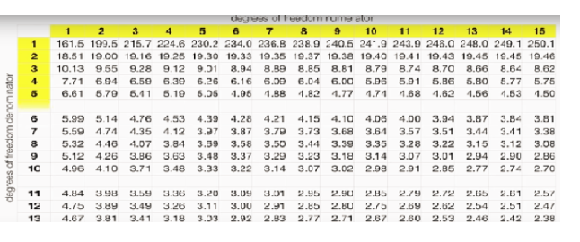
Degrees of freedom of the numerator will be that of the df between the groups.
Degrees of freedom of the denominator will be that of the df within the group.

The intersection will give us the critical F-value. Now, you compare your calculated F-value with the critical F-value.

• If calculated F < critical F, you will accept the null hypothesis.
• If calculated F > critical F, you will reject the null hypothesis.

Let’s now do the final calculations in your case to see whether Amazon, Flipkart and Snapdeal are equally popular:

Your critical F-value is 3.3690 and your calculated value comes out to be 4.78. Therefore, you will reject the null hypothesis and accept the alternate hypothesis. Therefore, Amazon, Flipkart and Snapdeal are not equally popular.