Time-series forecasting

Forecasting

It is the technique to predict future data analysing historical data.

Type of forecasting

Quantitative forecasting	Qualitative forecasting
Based on the data and any repeating historical patterns in the data.	This procedure is taken when data is not available and historical patterns do not repeat. This is based on expert decision.
Captures complex patterns which humans cannot identify.	May not capture complex patterns.
No bias	Bias
Eg. Time-series forecasting	Eg. Delphi method

Terminologies

• Time-series data: The data that has a time-component involved in it is termed as a time-series data. For ex: the number of orders made on a food ordering app per day is a time-series data.
• Time-series analysis: Analysis on the time-series data to find useful insights and patterns is termed as time-series analysis. For ex: In a food ordering app example, it might have the data for every day logged in per hour. They might notice that in this data, the number of orders is significantly higher in, say, the 1-2 PM time slot but is significantly lower in the 3-4 PM time slot. This information might be useful for them as they would then be able to estimate the number of delivery boys required at a particular time of the day. Hence, time series analysis is indispensable while working with any time series data.
• Time-series forecasting: It is basically looking at the past data to make predictions into the future. Say that the food ordering app wants to predict the number of orders per day for the next month in order to plan the resources better. For this, they will look at tons of past data and use it in order to forecast accurately.

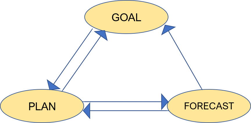
• Goal: A set of business objectives. For example, maximising revenue, maximising capital, etc.
• Plan: A set of actions that a business takes to achieve the goal. In order to come up with a good plan, they need a forecast.
• Forecast: Is the prediction of the future.

Problem statement: Air Passenger Traffic Forecasting problem

An airline company has the data on the number of passengers that have travelled with them on a particular route for the past few years. Using this data, they want to see if they can forecast the number of passengers for the next twelve months.
Making this forecast could be quite beneficial to the company as it would help them take some crucial decisions like:

• What capacity aircraft should they use?
• When should they fly?
• How many air hostesses and pilots do they need?
• How much food should they stock in their inventory?

Basic steps involved in any forecasting

• Define the problem
• Collect the data
• Analyze the data
• Build and evaluate forecast model

1. Define the problem

This is a crucial step in any Time-series forecasting or for that matter any type of analysis. We have to define and understand the problem well because if analysts doesn’t define the problem (or goal) then it can be difficult to analyse the final outcome. We can divide our process into following, or what to forecast?

• Quantity: Unit of problem to be forecasted. For ex: no. of units to sell, maximum occupancy to achieve, etc.
• Granularity: Scope of forecasting. For ex: analysis at store level, region level or city level, etc.
• Frequency: How frequent forecasting needs to be done? For ex: Daily basis, weekly basis, monthly, etc.
• Horizon: Is it Short-term, medium-term or long-term forecasting?

There are some caveats while performing Time-series forecasting:

• The Granularity rule: The more aggregate your forecasts, more accurate you are in your predictions. It is because aggregate data has lesser variance and hence, less noise.
• The Frequency rule: This rule tells you to keep updating your forecasts regularly to capture any new information that comes in.
• The Horizon rule: When you have the horizon planned for large number of months in the future, then you are more likely to be more accurate in your earlier months forecasts as compared to the later months.

Now that you have understood the steps in defining the problem, let’s apply them to the air passenger traffic problem.

• Quantity: Number of passengers
• Granularity: Flights from city A to city B; i.e., flights for a particular route
• Frequency: Monthly
• Horizon: 1 year (12 months)

2. Collect the data

It is very important because all your forecast is dependent on the data. There are three important characteristics that every time series data must exhibit in order for us to make a good forecast.

• Relevant: The time-series data should be relevant for the set objective that we want to achieve.
• Accurate: The data should be accurate in terms of capturing the timestamps and capturing the observation correctly.
• Long enough: The data should be long enough to forecast. This is because it is important to identify all the patterns in the past and forecast which patterns repeat in the future.

There are the various types of data sources to get a time-series data, which are:

• Private enterprise data: E.g. financial information about the quarterly results of any private organisation.
• Public data: E.g. government publishes the economic indicators such as GDP, consumer price index etc.
• System/Sensor data: E.g. Logs generated by the servers during their 24/7 working hours.

3. Analyze the data

There are components associated with time series, which are:

• Level: This is the baseline of a time series. This gives the baseline to which we add the different other components.

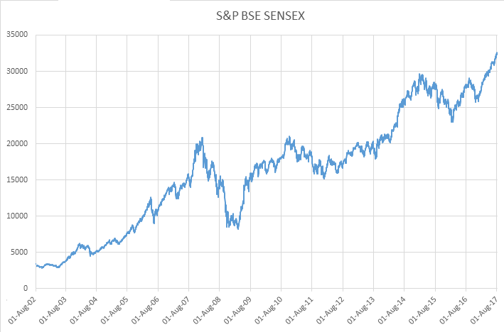
• Trend: Over a longterm, this gives an indication of whether the time series moves lower or higher. For example, in the following Sensex graph you can clearly observe that with time, the overall value is increasing i.e. this particular time series data has an increasing trend.

  

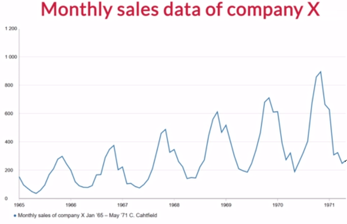
• Seasonality: It is a pattern in a time-series data that repeats itself after a given period of time. For example, in the following graph ‘Monthly sales data of company X’, you can clearly observe that a fixed pattern is repeating every year. The simplest example to explain this could be, say, the sales of winter wear in India. In winter, during months like November-January, you would expect these sales to be very high whereas for the other months, the sales might be low. This shows a seasonality pattern and proves to be very useful when making forecasts.

  

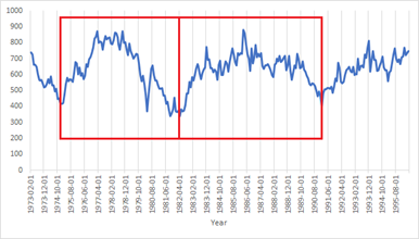
• Cyclicity: It is also a repeating pattern in data that repeats itself aperiodically. Read more about cyclicity here

  

• Noise: Noise is the completely random fluctuation present in the data and we cannot use this component to forecast into the future. This is that component of the time series data that no one can explain and is completely random.

  

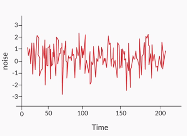
Note: Every time-series data has “Level” and “Noise” components compulsory, whereas other components are optional.

Handling missing values in time-series data

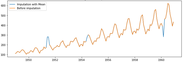
1. Mean imputation: Imputing the missing values with the overall mean of the data.
2. Last observation carried forward: We impute the missing values with its previous value in the data.
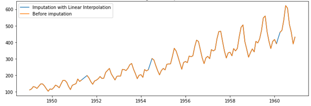
3. Linear interpolation: You draw a straight line joining the next and previous points of the missing values in the data.
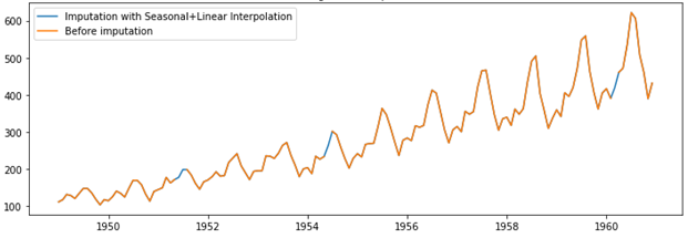
4. Seasonal + Linear interpolation: This method is best applicable for the data with trend and seasonality. Here, the missing value is imputed with the average of the corresponding data point in the previous seasonal period and the next seasonal period of the missing value.

Handling outliers in time-series data

Outliers are the data points within time-series which are way-off than expected data points. These may occur due to false readings or rare event.

We can detect and treat outliers in the time-series with following methods:

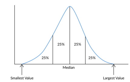
1. Extreme value analysis: Remove smallest and largest values in the dataset.
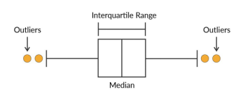
2. Box plot: The points lying on either side of whiskers are considered to be outliers. The length of whiskers can be defined by us according to the problem.
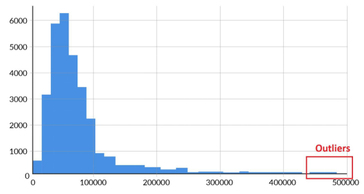
3. Histogram: Simply plotting a histogram can also reveal the outliers - basically the extreme values with low frequencies visible in the plot.

4. Build and evaluate the forecast models

Before modelling the data, time series need to be decomposed which can be done in two ways:

• Additive Seasonal Decomposition When the magnitude of the seasonal pattern in the data does not directly correlate with the value of the series, the additive seasonal decomposition may be a better choice to split the time series so that the residual does not have any pattern.
• Multiplicative Seasonal Decomposition When the magnitude of the seasonal pattern in the data increases with an increase in data values and decreases with a decrease in the data values, the multiplicative seasonal decomposition may be a better choice.

To build a model and forecast, we use Smoothing techniques. Smoothing techniques remove the noise components and retain the systematic patterns of the time series i.e. level, trend and seasonality.

There are differences between Time-series and Regression:

• Time-series have a strong temporal (time-based) dependence - each of these data sets essentially consists of a series of time-stamped observations i.e. each observation is tied to a specific time instance. Thus, unlike regression, the order of the data is important in a time-series.
• In a time-series, you are not concerned with the causal relationship between the response and explanatory variables. The cause behind the changes in the response variable is very much a black box.

Forecasting methods

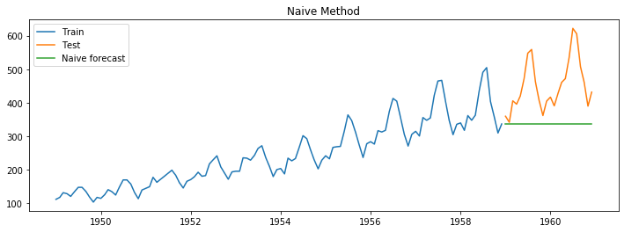
1. Naive method

   Forecast = Last month sales

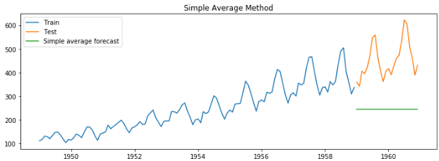
2. Simple average method

   Forecast = Average of all past months’ sales

Error measures

Following are the error measures in Time-series forecasting:

1. Mean Forecast Error (MFE): In this naive method, you simply subtract the actual values of the dependent variable, i.e., ‘y’ with the forecasted values of ‘y’. This can be represented using the equation below.
   $MFE = \dfrac{1}{n}\sum_{i=1}^n (y_{actual} - \widehat{y}_{forecast})$
2. Mean Absolute Error (MAE): Since MFE might cancel out a lot of overestimated and underestimated forecasts, hence measuring the mean absolute error or MAE makes more sense as in this method, you take the absolute values of the difference between the actual and forecasted values.
   $MAE = \dfrac{1}{n}\sum_{i=1}^n |y_{actual} - \widehat{y}_{forecast}|$
3. Mean Absolute Percentage Error (MAPE): The problem with MAE is that even if you get an error value, you have nothing to compare it against. For example, if the MAE that you get is 1.5, you cannot tell just on the basis of this number whether you have made a good forecast or not. If the actual values are in single digits, this error of 1.5 is obviously high but if the actual values are, say in the order of thousands, an error of 1.5 indicates a good forecast. So in order to capture how the forecast is doing based upon the actual values, you evaluate mean absolute error where you take the mean absolute error (MAE) as the percentage of the actual values of ‘y’.
   $MAPE = \dfrac{100}{n}\sum_{i=1}^n \vert\dfrac{y_i - \widehat{y}_i}{y_i}\vert$
4. Mean Squared Error (MSE): The idea behind mean squared error is the same as mean absolute error, i.e., you want to capture the absolute deviations so that the negative and positive deviations do not cancel each other out. In order to achieve this, you simply square the error values, sum them up and take their average. This is known as mean squared error or MSE which can be represented using the equation below.
   $MSE = \dfrac{1}{n}\sum_{i=1}^n (y_{actual} - \widehat{y}_{predicted})^2$
5. Root Mean Squared Error (RMSE): Since the error term you get from MSE is not in the same dimension as the target variable ‘y’ (it is squared), you deploy a metric known as RMSE wherein you take the square root of the MSE value obtained.
   $RMSE = \sqrt{\dfrac{1}{n}\sum_{i=1}^n (y_{actual} - \widehat{y}_{predicted})^2}$