Linear Regression: A Comprehensive Guide

Introduction
Mathematical Foundation
Types of Linear Regression
Algorithm Implementation
Assumptions
Evaluation Metrics
Advantages and Disadvantages
Common Interview Questions
Practical Considerations
Code Examples

Introduction

Linear Regression is one of the most fundamental and widely-used algorithms in machine learning and statistics. It models the relationship between a dependent variable (target) and one or more independent variables (features) using a linear equation. Despite its simplicity, it serves as the foundation for understanding more complex algorithms and remains highly effective for many real-world problems.

Key Concepts:

Supervised Learning: Uses labeled training data
Regression Task: Predicts continuous numerical values
Parametric Model: Assumes a specific functional form
Linear Relationship: Models linear relationships between variables

Mathematical Foundation

Simple Linear Regression

For a single feature, the linear regression model is:

\[y = \beta_0 + \beta_1 x + \epsilon\]

Where:

$y$ = dependent variable (target)
$x$ = independent variable (feature)
$\beta_0$ = y-intercept (bias term)
$\beta_1$ = slope (weight/coefficient)
$\epsilon$ = error term (noise)

Multiple Linear Regression

For multiple features, the model extends to:

\[y = \beta_0 + \beta_1 x_1 + \beta_2 x_2 + ... + \beta_n x_n + \epsilon\]

In matrix form:

\[\mathbf{y} = \mathbf{X}\boldsymbol{\beta} + \boldsymbol{\epsilon}\]

Where:

$\mathbf{y}$ = vector of target values $(n \times 1)$
$\mathbf{X}$ = design matrix of features $(n \times (p+1))$
$\boldsymbol{\beta}$ = vector of coefficients $((p+1) \times 1)$
$\boldsymbol{\epsilon}$ = error vector $(n \times 1)$
$p$ = number of features

Cost Function

The goal is to minimize the Mean Squared Error (MSE):

\[J(\boldsymbol{\beta}) = \frac{1}{2m} \sum_{i=1}^{m} (h_{\boldsymbol{\beta}}(x^{(i)}) - y^{(i)})^2\]

Where:

$m$ = number of training examples
$h_{\boldsymbol{\beta}}(x^{(i)}) = \boldsymbol{\beta}^T x^{(i)}$ = hypothesis function

In matrix form:

\[J(\boldsymbol{\beta}) = \frac{1}{2m} (\mathbf{X}\boldsymbol{\beta} - \mathbf{y})^T (\mathbf{X}\boldsymbol{\beta} - \mathbf{y})\]

Analytical Solution (Normal Equation)

The optimal parameters can be found analytically:

\[\boldsymbol{\beta} = (\mathbf{X}^T\mathbf{X})^{-1}\mathbf{X}^T\mathbf{y}\]

Conditions for existence:

$\mathbf{X}^T\mathbf{X}$ must be invertible (non-singular)
Number of features $<$ number of samples
Features must be linearly independent

Types of Linear Regression

1. Ordinary Least Squares (OLS)

Standard linear regression
Minimizes sum of squared residuals
No regularization

2. Ridge Regression (L2 Regularization)

Cost function with L2 penalty:

\[J(\boldsymbol{\beta}) = \frac{1}{2m} \sum_{i=1}^{m} (h_{\boldsymbol{\beta}}(x^{(i)}) - y^{(i)})^2 + \lambda \sum_{j=1}^{n} \beta_j^2\]

Where $\lambda$ is the regularization parameter.

3. Lasso Regression (L1 Regularization)

Cost function with L1 penalty:

\[J(\boldsymbol{\beta}) = \frac{1}{2m} \sum_{i=1}^{m} (h_{\boldsymbol{\beta}}(x^{(i)}) - y^{(i)})^2 + \lambda \sum_{j=1}^{n} |\beta_j|\]

4. Elastic Net

Combines L1 and L2 regularization:

\[J(\boldsymbol{\beta}) = \frac{1}{2m} \sum_{i=1}^{m} (h_{\boldsymbol{\beta}}(x^{(i)}) - y^{(i)})^2 + \lambda_1 \sum_{j=1}^{n} |\beta_j| + \lambda_2 \sum_{j=1}^{n} \beta_j^2\]

Algorithm Implementation

Gradient Descent Algorithm

ALGORITHM: Linear Regression with Gradient Descent

INPUT: 
  - Training data: X (m × n), y (m × 1)
  - Learning rate: α
  - Number of iterations: max_iter
  - Convergence threshold: ε

OUTPUT: Optimal parameters β

PROCEDURE:
1. Initialize β randomly or to zeros
2. Add bias column to X (column of ones)
3. FOR iteration = 1 to max_iter:
   a. Compute predictions: ŷ = X × β
   b. Compute cost: J = (1/2m) × ||ŷ - y||²
   c. Compute gradients: ∇J = (1/m) × X^T × (ŷ - y)
   d. Update parameters: β = β - α × ∇J
   e. IF ||∇J|| < ε: BREAK (convergence)
4. RETURN β

COMPLEXITY:
- Time: O(max_iter × m × n)
- Space: O(m × n)

Normal Equation Algorithm

ALGORITHM: Linear Regression with Normal Equation

INPUT: 
  - Training data: X (m × n), y (m × 1)

OUTPUT: Optimal parameters β

PROCEDURE:
1. Add bias column to X (column of ones)
2. Compute X^T × X
3. Check if X^T × X is invertible
4. IF invertible:
   a. Compute β = (X^T × X)^(-1) × X^T × y
5. ELSE:
   a. Use pseudo-inverse or regularization
6. RETURN β

COMPLEXITY:
- Time: O(n³) for matrix inversion
- Space: O(n²)

Assumptions

Linear regression relies on several critical assumptions that must be satisfied for the model to produce reliable and valid results. Violating these assumptions can lead to biased estimates, incorrect confidence intervals, and poor predictive performance.

1. Linearity

Definition: The relationship between the independent variables (features) and the dependent variable (target) is linear. This means the change in the target variable is proportional to the change in the feature variables.

Mathematical Expression: $E[Y|X] = \beta_0 + \beta_1 X_1 + \beta_2 X_2 + ... + \beta_p X_p$

Detailed Explanation:

The conditional expectation of Y given X follows a linear function
The coefficients represent the expected change in Y for a unit change in each X
Non-linear relationships cannot be captured without transformation

Consequences of Violation:

Biased coefficient estimates
Poor model fit and predictions
Incorrect interpretation of relationships

Detection Methods:

Scatter plots: Plot each feature against the target
Residual plots: Plot residuals vs. fitted values (should show random pattern)
Added-variable plots: Partial regression plots for each variable

Solutions when violated:

Polynomial features: $X^2, X^3, \sqrt{X}, \log(X)$
Interaction terms: $X_1 \times X_2$
Non-linear models: Decision trees, neural networks, kernel methods

2. Independence of Observations

Definition: Each observation in the dataset is independent of all other observations. The residual of one observation should not be predictable from the residuals of other observations.

Mathematical Expression: $Cov(\epsilon_i, \epsilon_j) = 0 \text{ for all } i \neq j$

Detailed Explanation:

No temporal correlation (autocorrelation)
No spatial correlation
No clustering effects
Random sampling from the population

Consequences of Violation:

Underestimated standard errors
Overconfident statistical tests
Inefficient parameter estimates
Poor generalization

Common Violations:

Time series data: Sequential observations are correlated
Clustered data: Students within schools, patients within hospitals
Spatial data: Geographic proximity creates correlation

Detection Methods:

Durbin-Watson test: Tests for first-order autocorrelation
Ljung-Box test: Tests for higher-order autocorrelation
Residual plots: Plot residuals vs. observation order
ACF/PACF plots: Autocorrelation and partial autocorrelation functions

Solutions when violated:

Generalized Least Squares (GLS)
Mixed-effects models for clustered data
Time series models (ARIMA, VAR)
Robust standard errors (Newey-West)

3. Homoscedasticity (Constant Variance)

Definition: The variance of the residuals is constant across all levels of the independent variables. The spread of residuals should be the same regardless of the predicted values.

Mathematical Expression: $Var(\epsilon_i) = \sigma^2 \text{ for all } i$

Detailed Explanation:

Residual variance doesn’t depend on X values
Error terms have uniform spread
No “funnel” or “fan” patterns in residual plots

Consequences of Violation (Heteroscedasticity):

Inefficient parameter estimates (still unbiased)
Incorrect standard errors and confidence intervals
Invalid hypothesis tests
Suboptimal predictions

Detection Methods:

Residual plots: Plot residuals vs. fitted values
Breusch-Pagan test: Statistical test for heteroscedasticity
White test: More general test for heteroscedasticity
Goldfeld-Quandt test: Compares variances in subgroups

Solutions when violated:

Weighted Least Squares (WLS): Weight observations by inverse variance
Robust standard errors: Huber-White sandwich estimators
Transformation: Log, square root, or Box-Cox transformations
Generalized Least Squares: Model the variance structure

4. Normality of Residuals

Definition: The residuals (error terms) are normally distributed with mean zero. This assumption is crucial for hypothesis testing and confidence intervals.

Mathematical Expression: $\epsilon_i \sim N(0, \sigma^2)$

Detailed Explanation:

Residuals follow a normal distribution
Mean of residuals is zero
Required for statistical inference (t-tests, F-tests)
Less critical for large samples (Central Limit Theorem)

Consequences of Violation:

Invalid confidence intervals
Incorrect p-values and hypothesis tests
Suboptimal predictions (though estimates remain unbiased)
Problems with small samples

Detection Methods:

Q-Q plots: Quantile-quantile plots against normal distribution
Shapiro-Wilk test: Tests normality of residuals
Anderson-Darling test: More sensitive to tail behavior
Kolmogorov-Smirnov test: General goodness-of-fit test
Histogram of residuals: Visual inspection

Solutions when violated:

Transformation: Box-Cox, log, square root transformations
Robust regression: Huber, bisquare, or other M-estimators
Non-parametric methods: Bootstrap confidence intervals
Different distributions: Generalized Linear Models (GLMs)

5. No Multicollinearity

Definition: The independent variables are not highly correlated with each other. Each feature should provide unique information about the target variable.

Mathematical Expression: Perfect multicollinearity: $X_j = \alpha + \beta X_k$ for some features j and k

Detailed Explanation:

Features should be linearly independent
No exact or near-exact linear relationships between predictors
Each feature contributes unique information
Correlation matrix should not have values close to ±1

Consequences of Violation:

Unstable coefficient estimates
Large standard errors
Difficulty interpreting individual coefficients
Numerical instability in matrix inversion
Poor model generalization

Types of Multicollinearity:

Perfect: Exact linear relationship (matrix is singular)
High: Near-linear relationship (numerical problems)
Moderate: Some correlation but manageable

Detection Methods:

Correlation matrix: Pairwise correlations between features
Variance Inflation Factor (VIF): $VIF_j = \frac{1}{1-R_j^2}$
- VIF > 5: Moderate multicollinearity
- VIF > 10: High multicollinearity
Condition Number: Ratio of largest to smallest eigenvalue
Tolerance: $1/VIF$ (values < 0.1 indicate problems)

Solutions when violated:

Remove redundant features: Drop highly correlated variables
Principal Component Analysis (PCA): Create orthogonal components
Ridge regression: L2 regularization handles multicollinearity
Partial Least Squares (PLS): Combines features optimally
Domain knowledge: Choose most relevant features

Assumption Validation with Python Examples

Here’s comprehensive Python code to check all assumptions with visualizations:

Linear Regression Assumptions Validation Code

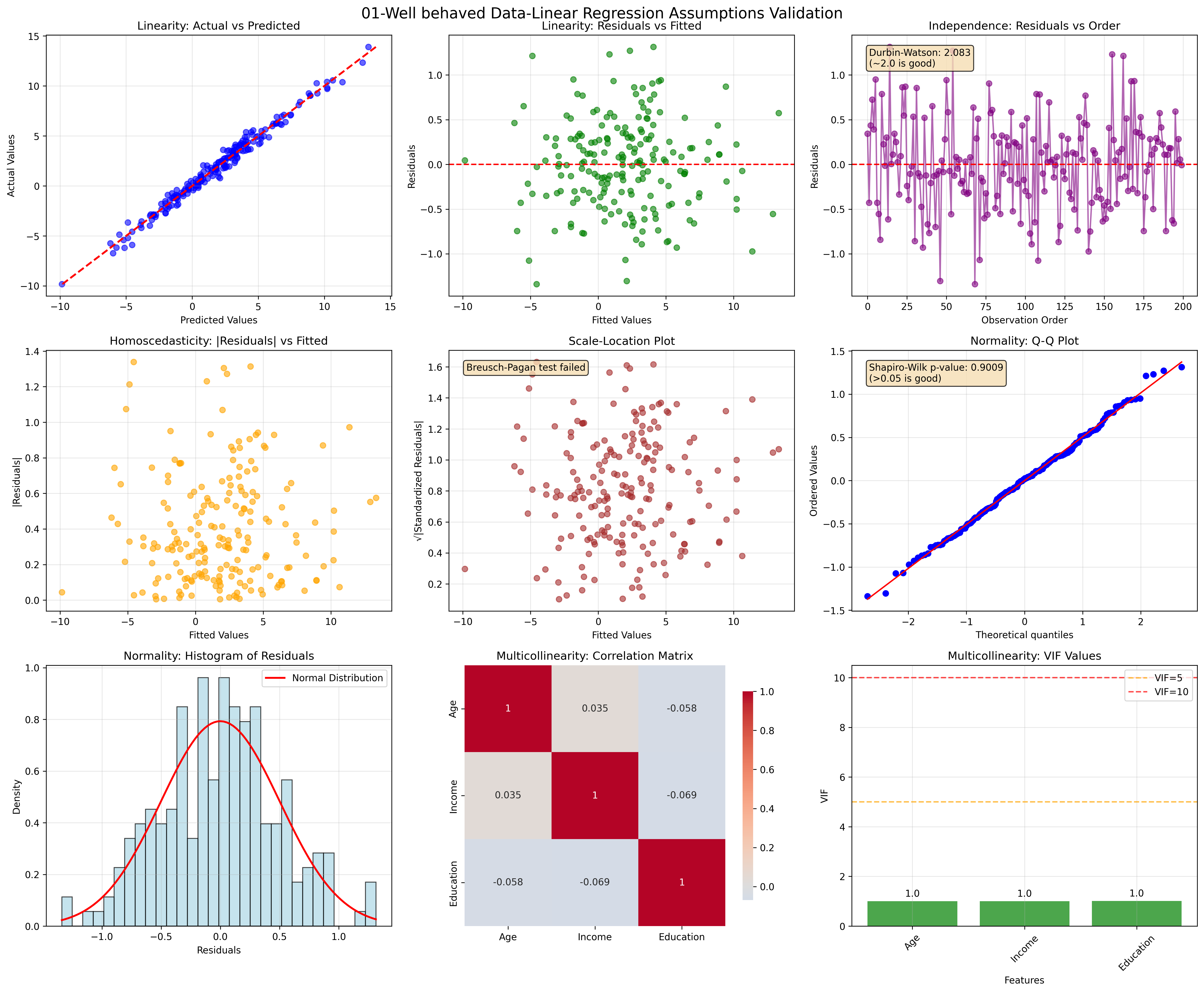
This comprehensive code provides:

Visual diagnostics for all five assumptions
Statistical tests with interpretation guidelines
Example datasets showing different violation scenarios
Color-coded warnings for problematic values
Summary statistics with actionable insights

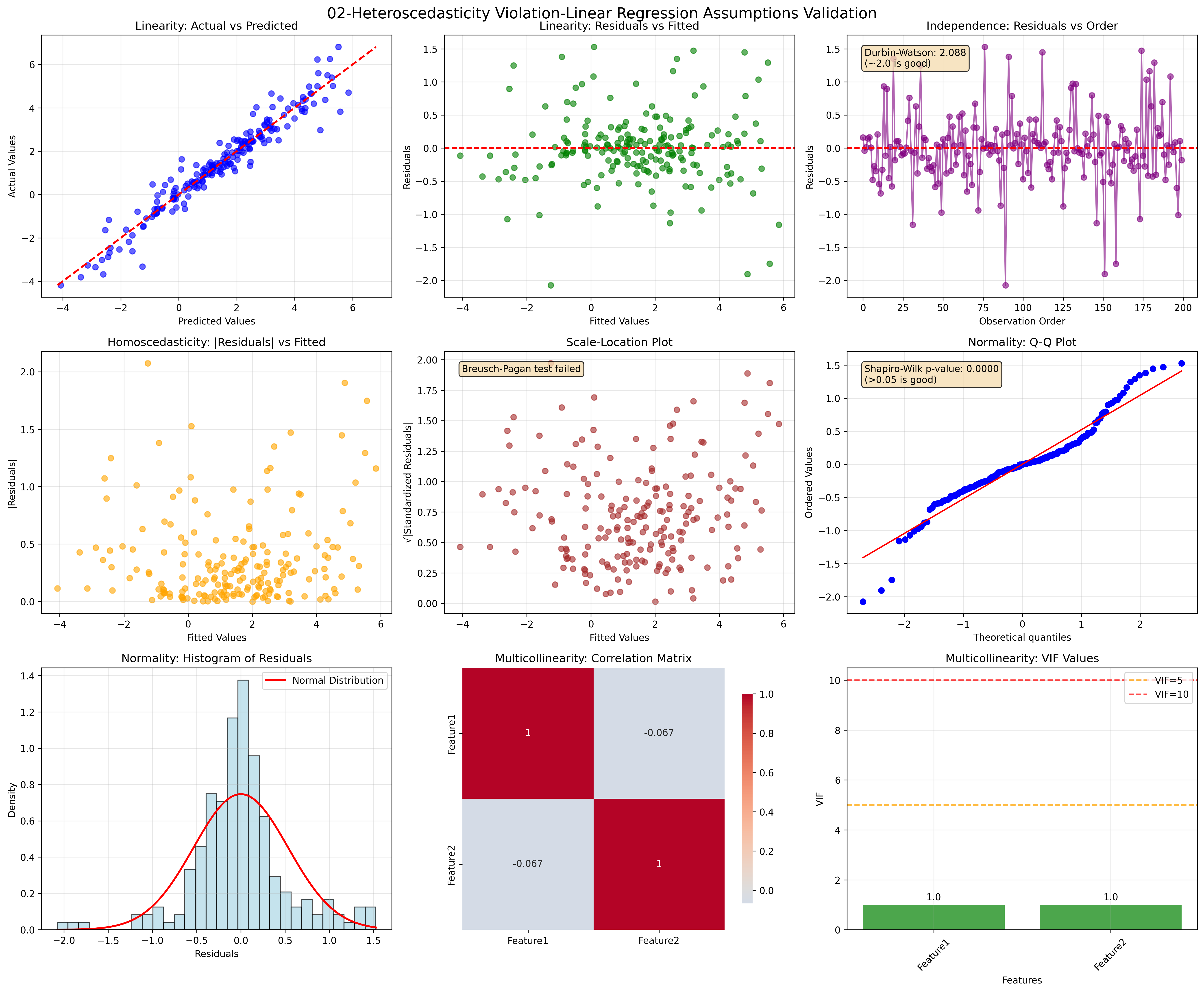
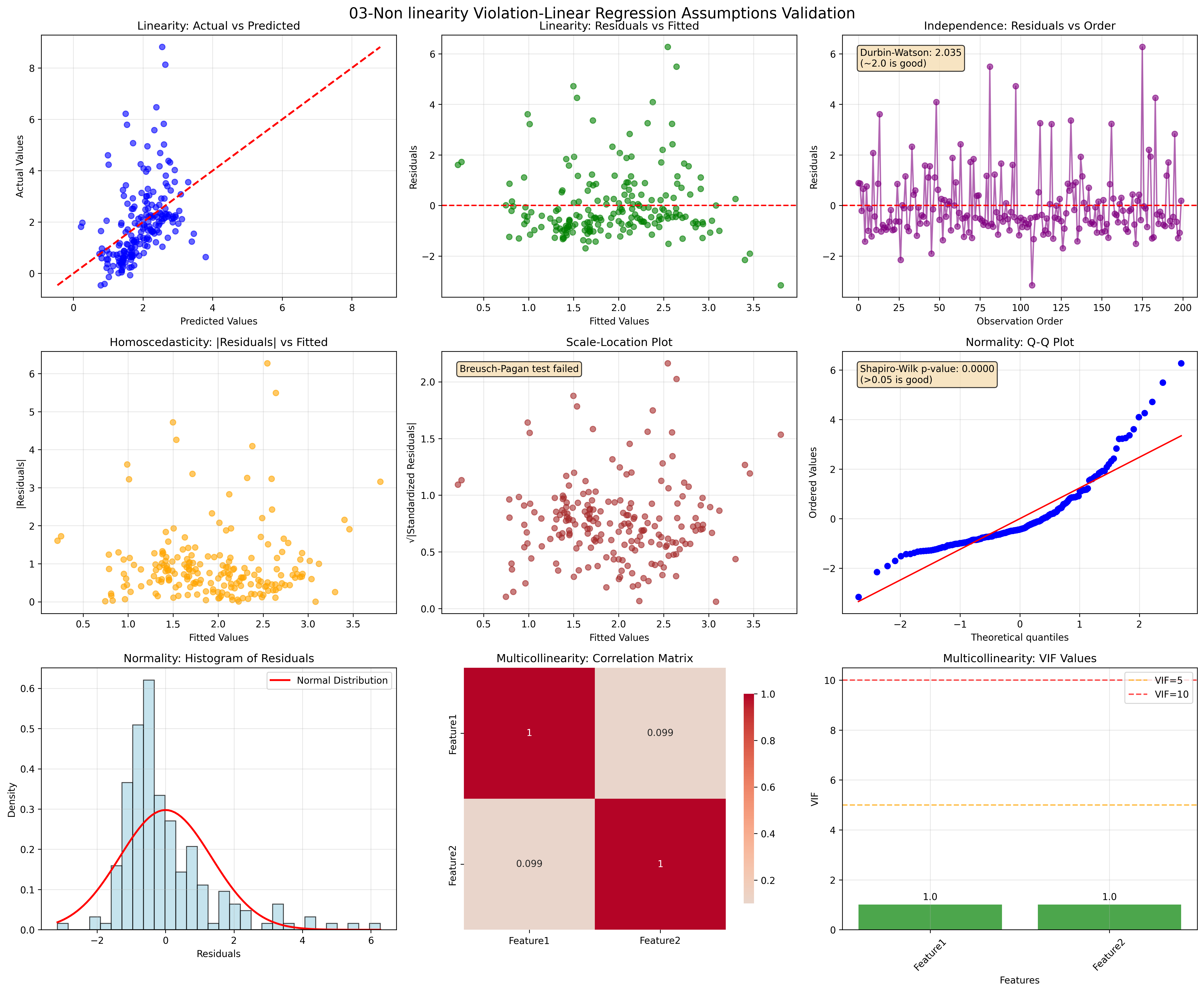
The graphs generated will clearly show:

Linearity: Scatter plots and residual patterns
Independence: Autocorrelation patterns and Durbin-Watson statistics
Homoscedasticity: Variance patterns and statistical tests
Normality: Q-Q plots, histograms, and normality tests
Multicollinearity: Correlation heatmaps and VIF values

Following are the generated graphs for different scenarios:

01. Well-behaved Data

02. Heteroscedasticity Violation

03. Non-linearity Violation

Quick Reference for Assumption Checking

Assumption	Quick Check	Warning Signs	Solutions
Linearity	Residual plots	Curved patterns	Polynomial features, transformations
Independence	Durbin-Watson	DW ≠ 2.0	GLS, robust SE, time series models
Homoscedasticity	Residual spread	Funnel patterns	WLS, robust SE, transformations
Normality	Q-Q plots	Skewed residuals	Transformations, robust methods
No Multicollinearity	VIF values	VIF > 10	Remove features, PCA, Ridge regression

Evaluation Metrics

1. Mean Squared Error (MSE)

$MSE = \frac{1}{m} \sum_{i=1}^{m} (y_i - \hat{y}_i)^2$

2. Root Mean Squared Error (RMSE)

$RMSE = \sqrt{MSE}$

3. Mean Absolute Error (MAE)

$MAE = \frac{1}{m} \sum_{i=1}^{m} |y_i - \hat{y}_i|$

4. R-squared (Coefficient of Determination)

$R^2 = 1 - \frac{SS_{res}}{SS_{tot}} = 1 - \frac{\sum_{i=1}^{m} (y_i - \hat{y}_i)^2}{\sum_{i=1}^{m} (y_i - \bar{y})^2}$

5. Adjusted R-squared

$R^2_{adj} = 1 - \frac{(1-R^2)(m-1)}{m-p-1}$

Where $p$ is the number of features.

Advantages and Disadvantages

Advantages

Simplicity: Easy to understand and implement
Interpretability: Coefficients have clear meaning
Fast Training: Analytical solution available
No Hyperparameters: For basic OLS
Baseline Model: Good starting point for regression tasks
Low Variance: Stable predictions across different datasets

Disadvantages

Linearity Assumption: Cannot capture non-linear relationships
Sensitive to Outliers: Squared error penalty
Multicollinearity: Performance degrades with correlated features
Feature Scaling: Requires normalization for gradient descent
Overfitting: With many features relative to samples
Homoscedasticity: Assumes constant variance

Common Interview Questions

Technical Questions

Q: What is the difference between Ridge and Lasso regression?
- Ridge: Uses L2 regularization, shrinks coefficients toward zero but doesn’t set them to exactly zero
- Lasso: Uses L1 regularization, can set coefficients to exactly zero (feature selection)
Q: When would you use gradient descent vs. normal equation?
- Gradient Descent: Large datasets (m > 10,000), when X^TX is not invertible
- Normal Equation: Small to medium datasets, when analytical solution is feasible
Q: How do you handle multicollinearity?
- Remove highly correlated features
- Use regularization (Ridge/Lasso)
- Principal Component Analysis (PCA)
- Variance Inflation Factor (VIF) analysis
Q: What if linear regression assumptions are violated?
- Non-linearity: Polynomial features, kernel methods
- Heteroscedasticity: Weighted least squares, robust standard errors
- Non-normality: Robust regression methods
- Autocorrelation: Generalized least squares

Coding Questions

Q: Implement linear regression from scratch
Q: How would you detect and handle outliers?
Q: Implement cross-validation for model selection

Practical Considerations

Feature Engineering

Polynomial Features: Capture non-linear relationships
Interaction Terms: Model feature interactions
Feature Scaling: Standardization or normalization
Feature Selection: Remove irrelevant features

Model Selection

Cross-Validation: K-fold, stratified sampling
Information Criteria: AIC, BIC for model comparison
Regularization Path: Grid search for optimal λ

Diagnostics

Residual Analysis: Check assumptions
Influence Measures: Cook’s distance, leverage
Collinearity Diagnostics: VIF, condition number

Code Examples

Python Implementation from Scratch

Linear Regression from Scratch Code

Regularized Linear Regression

Ridge Regression from Scratch Code

Back to ML Algorithms

Back to Home

Linear Regression: A Comprehensive Guide

Table of Contents

Introduction

Mathematical Foundation

Simple Linear Regression

Multiple Linear Regression

Cost Function

Analytical Solution (Normal Equation)

Types of Linear Regression

1. Ordinary Least Squares (OLS)

2. Ridge Regression (L2 Regularization)

3. Lasso Regression (L1 Regularization)

4. Elastic Net

Algorithm Implementation

Gradient Descent Algorithm

Normal Equation Algorithm

Assumptions

1. Linearity

2. Independence of Observations

3. Homoscedasticity (Constant Variance)

4. Normality of Residuals

5. No Multicollinearity

Assumption Validation with Python Examples

Quick Reference for Assumption Checking

Evaluation Metrics

1. Mean Squared Error (MSE)

2. Root Mean Squared Error (RMSE)

3. Mean Absolute Error (MAE)

4. R-squared (Coefficient of Determination)

5. Adjusted R-squared

Advantages and Disadvantages

Advantages

Disadvantages

Common Interview Questions

Technical Questions

Coding Questions

Practical Considerations

Feature Engineering

Model Selection

Diagnostics

Code Examples

Python Implementation from Scratch

Regularized Linear Regression